
Minia Assembler and French Revolution
**What is more challenging than understanding computer code written by someone, who is very intelligent?
Ans. Figuring out computer code written by someone, who is very intelligent and thinks in French :)**
Over the last few days, we have been working hard to understand Minia assembly algorithm of Rayan Chikhi and Guillaume Rizk. We started with two sources - (i) their paper and (ii) their C++ code, which Rayan kindly provided to us. We picked Minia, because its code-base is short, but it still completes the assembly in an efficient manner (see slides). So, Minia is a good example for learning how a modern genome assembler works. Please note that Minia is only a contig assembler. It completes the first stage of the assembly to combine short reads into small nucleotide regions called contigs (average length 1K). However, that first step is the most memory intensive for most NGS libraries.
The paper itself is well written for anyone interested in getting some sense of the algorithm, and there is no need to sift through the code. Our intention was to know it so well that we could implement the code from scratch, even if we were stranded in an empty tropical islands with only our laptops. For most bioinformatics algorithms, that level of understanding cannot be developed without going through the codes, because many small details are usually not provided in papers. For example, questions like which data structures are used to optimize different steps, which hash functions form Bloom filter, how data- flow between memory and hard disk is optimized, etc. cannot be fully explained in four or five page papers. Previously, we went through the same exercise of studying the code for Velvet, and the experience had been rewarding.
To make our life more difficult, we decided to figure out the code without seeking any help from Rayan. That was a bad decision, because we got stuck on the first page of the simplest class.
#define TAILLE_NOM 1024
What is the meaning of name ‘TAILLE_NOM’? A tax by ancien regime imposed on peasants? We do not speak French, and being history buff made our life even more difficult. With help from a dictionary, we figured out that ‘TAILLE’ means size and name of another important graph function ‘avance’ means advance. After few more hiccups, we were set to go.

History of development
Before we continue, let us present the history of Minia. It belongs to what we call second generation assembly algorithms for NGS libraries. Speaking of historical developments -
i) Velvet-like de Bruijn assemblers: The first generation algorithms (e.g. Velvet, SOAPdenovo) were developed to show the feasibility of de novo assembly from short reads, because at that point it was not clear, whether short reads could be assembled into genomes. That problem was solved, but researchers noticed that the algorithms did not scale well for large genomes. SOAPdenovo needed 512GB RAM to assemble the panda genome.
ii) K-mer counting and filtering: Researchers figured out that scaling of algorithms could be improved by counting k-mers and removing low-frequency k-mers. However, the k-mer counting algorithms themselves posed scaling challenges for large libraries. Bloom filter-based algorithms showed the best memory performance.
iii) Bloom filter-based filtering algorithms: CTB’s group went one step further to use Bloom filters to remove redundant reads as part of an one-step library reduction algorithm. The reduced library was fed into traditional assemblers like Velvet, and were expected to assemble as well as the full library.
iv) Minia - an assembler that uses Bloom filter to hold its k-mers: When the paper from Pell et al. was posted at arxiv, Rayan was working hard to develop memory-efficient assemblers. He incorporated Bloom filter within his de Bruijn graph assembler as the data structure for ‘storing’ k-mers, and showed that his assembler could complete human assembly with enough RAM available in a typical desktop computer. No big server was needed anymore.
Class structure
Let us start with discussing the class structure of Minia.

The code consists of seven relatively simple class files, two complex class files closely related to genome assembly and the main program ‘assembly.cpp’, which is long with multiple big functions. When we use the word ‘big or ‘complex’ for a function, we use ‘standard definition’ as explained here (slightly modified) :) -
A friend of mine was once interviewing an engineer for a programming job and asked him a typical interview question: how do you know when a function or method is too complex? Well, said the candidate, I don’t like any method to be bigger than my head. You mean you can’t keep all the details in your head? No, I mean I put my head up against my monitor, and the code shouldn’t be bigger than my head.
All functions in Bank, Bloom, Hash16, Kmer, Pool, Set and LinearCounter class files were smaller than our heads. Terminator class had one function (constructor of ‘BranchingTerminator’) that was bigger, and so we call the class somewhat complex. Most functions in Terminator class file and assemble.cpp were large, and took several iterations to understand fully.
The Assembly Approach
Earlier, we wrote extensively on the basic working of de Bruijn graph-based assemblers (de Bruijn graphs - I, de Bruijn graphs - II, de Bruijn graphs - III, sequencing errors, a drawback of de bruijn graph approach). First generation assembly algorithms could be easily understood from those discussions, because they were straightforward implementations of de Bruijn graph-based approach with less thought on memory performance. Second generation algorithms, on the other hand, try to optimize every single step of assembly process to improve scalability. So, their novelties cannot be appreciated without going through the details of implementation in terms of data structures and data flow. Let us discuss the unique implementations in Minia.
a) Removal of edges: A mathematical graph consists of nodes and edges. De Bruijn graphs for genomic sequences are special in that respect, because one can get rid of edges completely and still store the graph. That simplification can lead to huge memory savings, because mathematically one is storing an array instead of a matrix.
Why is it possible to remove the edges and still be able to reconstruct the graph? Let us figure that out with an example.
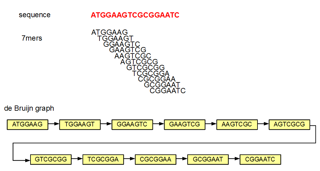
In the above figure of de Bruijn graph, each node and its neighbor differ by exactly one nucleotide. Let us say that you store the above de Bruijn graph in a hash. If you know that one node is TGGAAGT (second in the chain), you can query the hash by asking whether any of the four possible neighbors on the right side (GGAAGTA, GGAAGTC, GGAAGTG, GGAAGTT) and four possible neighbors on the left side (ATGGAAG, CTGGAAG, GTGGAAG, TTGGAAG) exist in the hash. If any of those neighbors exist, you know that they are linked in the graph, because de Bruijn graphs always link two nodes differing by exactly one nucleotide. So, you can essentially build the whole graph by knowing only the nodes or the k-mers.
The primary disadvantage of not storing the edges is that one needs to now find them out through eight queries. So, it is a straightforward issue of speed versus memory usage.
b) Error Correction Through Removal of Low Abundance K-mers:
After deciding to store only the k-mer nodes, Minia decided to do k-mer counting among all reads and use only those k-mers present three or more times in the NGS library for further analysis. This step effectively removes all spurious nodes and branches.
b) Genomic de Brijn Graphs Consist Mostly of Simple Chains and Few Branching Nodes:
After step (b), we are left with k-mers that mostly belong to the genome and de Bruijn graph they form is nearly identical to the de Bruijn graph of the genome. So, the question is how the de Bruijn graph of a genome looks like? We wrote extensively on that topic in the earlier commentaries, but just to give you some sense of it, let us draw a cartoon picture:

The above picture shows de Bruijn graph of a genome. All dashed lines in the picture are composed of hundreds of k-mer nodes, and those k-mers have exactly one left neighbor and one right neighbor. Only when the lines intersect or terminate, k-mers have different or more complex neighborhood patterns. Let us call them ‘branching nodes’. If you start traversing the graph from a non- branching k-mer and go to left or right along its line, your journey will always end at the same pair of branching nodes. Also note that, based on (a), traversing the graph means starting from a k-mer and checking whether its four possible left neighbors and four possible right neighbors exist in the graph.
Using above information, Minia formed an elegant graph traversal method for NGS de Bruijn graphs that did not require too much memory. In a typical graph traversal method, one needs to mark all nodes that are already reached. Since de Bruijn graphs have large number of non-branching nodes and small number of branching nodes, it is only necessary to store detailed information on the branching nodes. Alternatively, one can store information only on nodes immediately neighboring branching nodes (‘terminal nodes’). That cuts large amount of storage overhead for the graph traversal routine. Remember that Rayan put lot of thought in Minia to use as little RAM as possible.
In this context, also note that two lines intersecting in a de Bruijn graph does not always mean they represent some kind of repeat in the genome. Sometimes, two lines in a de Bruijn graph can have spurious overlaps that goes away with choice of longer k-mer.
d) Bloom Filters Store Approximate de Bruijn Graphs:
The genome assembly, following steps (a-c) can be completed by using a hash for storing the k-mers and another smaller data structure for branching or terminal nodes to store additional information (visited or not, etc.). Can we do better?
Hashes are memory intensive, and Bloom filters provide a memory-light alternative for storing k-mers. Bloom filters are bit arrays data structures with two functions - ‘insert’ and ‘does it exist’. The ‘insert’ function inserts a k-mer into Bloom filter, and you can put as many k-mers as possible. The ‘does it exist’ function tells you whether a k-mer is already inserted in a Bloom filter.
Why do Bloom filters save space compared to hashes? It is because, unlike hashes, they can sometimes give wrong answers. What good is a data structure, if it is prone to give wrong answers? The advantage of Bloom filters is that they can only give wrong answers in one direction. When you ask ‘does it exist’ for a k-mer, if the Bloom filter says no, the k-mer definitely does not exist in the Bloom filter. If it says yes, the answer may turn out to be false positive and the k-mer may or may not exist in the Bloom filter. The art here is to reduce the number of false positives or find a way around them.
The biggest contribution of Minia algorithm is its ability to devise an elegant way around the false positives. If you follow (a-c), you understand the general nature of their graph traversal algorithm. When the Bloom filter came into the picture, Minia team started to think about how the Bloom filter would introduce abnormalities in their graph traversal approach.
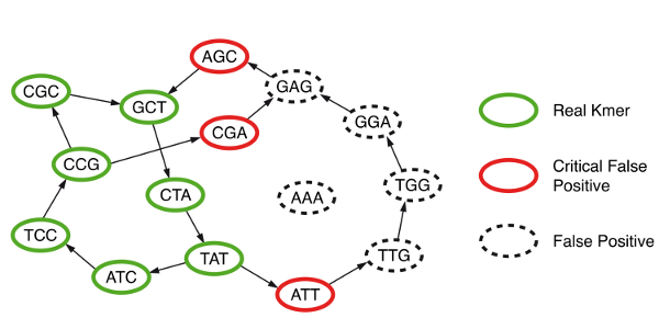
They discovered that, in addition to true branching nodes in their graph, Bloom filter would create false branching nodes (see figure below, hotlinked from Minia website). If those false branching nodes (or more generally ‘critical false positives’) were marked prior to traversing the graph and saved in a separate data structure, then an exact graph traversal algorithm as in (c) could be performed even though k-mers were stored in memory in faulty data structure (Bloom filter). The extra overhead for storing critical false positives was relatively small.
How can the false branching nodes created due to Bloom filter be marked? It was done through a 2-step process that required extensive use of the hard- drive. Please note that the real k-mers (‘solid k-mers’ of S) in the NGS library were already saved in the disk as a result of step (a). Minia picked each k-mer, asked whether any of its eight neighbors was present in the Bloom filter, and if it was present, the k-mer for the neighbor was saved in hard- drive in a new file (P). This was done for all real k-mers, and the resulting P file had all one-base extensions of solid k-mers that were also present in the Bloom filter.
As this stage, Minia had two large files in the hard-drive composed of real k-mers (S) and one base extensions of real k-mers (P). The ‘critical false positive’ set could be formed by subtracting S from P. Please note even though the difference of P and S is small, each file P and S is huge and cannot be loaded into memory all at once. Minia did the subtraction by loading S in memory part by part, going through the entire P file from hard drive and storing only those that did not have matches with S.
**Flow-chart of all steps with information on time/RAM **
The numbers in following chart are from Minia paper and related to assembly of human genome. Please note that
(i) one key objective of Minia was to bring memory usage down to typical desktop computers. So, the maximum memory usage at some steps are fixed at 4 Gb. Without that constraint, time performance will improve,
(ii) single core is used for each step. There is room for significant performance improvement, if parallelism is used.
